Last month’s post focused on how to best treat future energy or carbon savings and how this decision can affect whether short-term or long-term investments are more favorable. But even more crucial to the calculation is the persistence of the savings – that is, what savings can we expect in the future and for how long? What if a measure and its efficiency last well into the future but people begin to use that equipment or resource more, reducing or negating any savings?
Persistence
Whatever one’s reason for installing a new energy-efficient widget or implementing an energy-efficient behavior, the two most important pieces of information needed are what does it cost (usually in terms of money) and what are the benefits (usually in terms of energy savings or reductions in greenhouse gases). On the benefit side of the ledger, we need to understand the magnitude of the savings and how long those savings will last. We can quibble over how to discount future benefits, but the most important thing to know is that the savings actually last into the future for an expected period of time.
I am currently working on a few studies that, either directly or indirectly, investigate the persistence of energy efficiency measures and their savings. In other words, how long can we count on measures and savings to last?
Historically, energy efficiency programs have focused on first-year savings. When we want to understand how much the measure will save over its lifetime, we simply multiply the first-year savings by its effective useful life (EUL)[1]. Utilities are increasingly interested in the lifetime savings of measures for goal setting and this metric has always been needed for cost-effectiveness testing. This reflects a general trend of the industry becoming more mature and smarter. Program administrators are now less focused (hopefully) on hoarding every kWh of savings, even if it is short-term and does not help with peak demand (ahem, residential lighting), and are now focusing on deeper retrofits with long-lasting measures when the energy is saved and benefits beyond energy savings.
As I have covered before, EUL estimates are notoriously problematic and the values used are often based on ancient low rigor studies, unsourced estimates, and broad measure life edicts not based on the actual equipment.
While EUL is helpful in estimating the lifetime savings of a measure, what we are really interested in is the persistence of savings. We should be interested in whether in year 12 the heat pump is realizing 80% of its anticipated annual savings or only 20%.
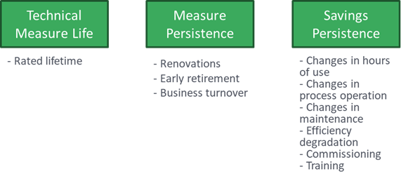
Overall savings persistence can be thought of as having three elements:
- Technical Measure Life: The rated lifetime (and related failures) that a piece of equipment can technically last in a lab
- Measure Persistence: A factor that accounts for real-life failures and other reasons why the measure may not be in use, such as early retirement, business turnover, remodeling/renovations, and storm damage
- Savings Persistence: A factor that accounts for changes to the facility/operations (e.g., changes to hours of operation), behavior (e.g., training, commissioning), and efficiency degradation[2]
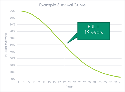
A measure’s persistence can be illustrated as a survival curve. At any given time, a certain percentage of measures are expected to have failed and a certain percentage are expected to have survived (so far). A measure’s EUL is the point when 50% of the measures are expected to have survived.
Often when conceptualizing persistence, I think that the maximum savings are achieved on the day of the program’s intervention and savings begin to evaporate every day after as equipment is not maintained, staff turnover occurs and valuable experience is lost, settings are reset, and equipment ages. In most cases, this is true. However, for some programs/measures, like strategic energy management (SEM), the intervention occurs continuously as opposed to a single point in time and can/should result in the continual improvement of the energy savings over time, complicating the persistence question.
If long-term energy savings are desired (and should be if we have any hope to mitigate climate change), then it is important to keep measure and savings persistence as close to 100% as possible. If that is not realistic, at the very least, we should research the real persistence of measures and savings so that we are not counting on future savings that will never materialize. In addition to this, though, we must be aware of a potential reduction in future savings due to increased usage of more efficient resources – the rebound effect.
Rebound Effect
In 1865, an economist named William Jevons observed that the higher efficiency of coal use (i.e., Watts’ steam engine) would increase rather than decrease Britain’s demand for coal. He argued that lowering the price of energy would increase demand and open up new ways to utilize coal. This is known as the Jevons paradox.
A more modern example of the Jevons paradox is the fuel efficiency of cars. Studies have found that increases in cars’ fuel efficiency lead to more miles driven (they checked people’s odometers). The rebound effect may be about 10%.[3]
This chart shows a simplified example. As we move from the baseline case to the efficient case, we expect to move from point A to point B and realize savings of the difference between E0 and E1 given the current level of energy service (e.g., hours of operation, miles traveled, etc.). But what can happen is that we actually arrive at point C because we increase our use of the service because of the lower energy bill. Note that this example shows a partial rebound effect in which the rebound effect decreases savings, but does not eliminate them. In Jevons’ paradox, a backfire effect occurs in which S1 would be way out to the right, making E2 above E0, increasing overall energy consumption.[4]
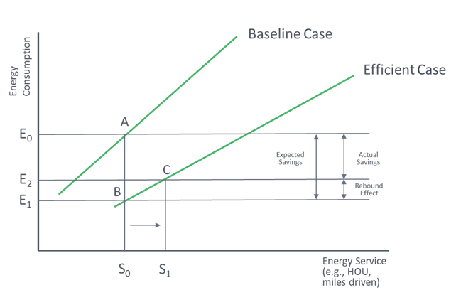
Adapted from this paper.
Most research on rebound effects (that I have seen) has focused on fuel efficiency in cars, but the rebound effect also occurs in other areas, like heating, cooling, and water heating. Estimates for the rebound effect for these end uses may be around 20%.
So far we have been covering direct rebound effects, which focuses on the individual household or firm’s increased use of the efficient service (e.g., turning up your thermostat because your heating bill is lower). But there can be indirect rebound effects as well in which the household or firm uses their increased income from the bill savings to buy other stuff which requires energy to make/use. The aggregate of the direct and indirect rebound effects can be large and are important to understand for decarbonization.[5]
Clean Energy Matters
One important consideration is that energy use on its own is not bad and therefore neither is the rebound effect. If the bill savings from having more efficient heat in their home allows someone to turn up their thermostat to keep their family warm, then it is a good outcome. In most places, access to energy is not an issue, but access to affordable energy may be. Increased energy usage can lead to many positive social and economic outcomes. The key is that the energy needs to be clean, which means that it needs to be electric and coming from carbon-free sources.
Given the challenges of decarbonization, efficiency is still the best way to reduce carbon emissions. If we are counting on energy efficiency to account for a large part of climate mitigation, we need to count lifetime savings accurately. This means that now more than ever, it is crucial to understand how long savings persist and the size of rebound effects.
[1] The median life of the measure, or how long it takes for 50% of the measures to fail.
[2] Note that the performance/efficiency of both baseline equipment and efficient equipment degrades over time, usually at close enough of the same rate. We really only care about the net degradation of efficient equipment compared to baseline equipment.
[3] This means that if fuel economy standards lead to the cost per mile decreasing by 5%, a rebound effect of 10% would mean that the number of miles driven will increase by 2%.
[4] The size of the rebound effect depends on the price elasticity of the resource, meaning how sensitive demand is to changes in price. In countries like the US, the demand for energy is relatively inelastic (e.g., it takes a pretty big change in the price of gas for us to significantly change the amount we drive), but the demand is more elastic in poorer countries.
[5] I saw a stat recently that savings from all electric energy efficiency programs in the US totaled 211 TWh in 2018. Meanwhile, the current (global) annualized Bitcoin energy consumption is estimated at 127 TWh!