As global average temperatures continue to rise due to climate change caused by humans, the amount of energy used (and potentially saved) cooling buildings will also increase. But if savings are calculated using outdated weather data that do not incorporate recent temperature increases, energy efficiency programs may be undercounting energy savings for cooling measures. This discrepancy becomes even more apparent when forecasting lifetime savings. Read on as we dive into weather data, cooling savings, and lots of acronyms!

It’s Getting Warmer
Like many, the recent extreme heat in the Pacific Northwest was eye-opening. I live on the other side of the country in Massachusetts and dealt with a high of 98°F that week and that was plenty hot enough. It is hard to fathom temperatures of 115°F with no air conditioning.[1] The terrifying thing is that these extreme weather conditions are likely to increase in regularity as global temperatures continue to inch upward due to human-induced climate change.
It made me think of the climate stripes, a simple yet scary graphic made by Ed Hawkins showing the relative change in global temperature from 1850-2020.[2] That graphic is so striking to me that it was one of my go-to masks during the pandemic.[3]
Energy-efficiency programs use weather data to calculate loads for weather-dependent measures (e.g., HVAC equipment and insulation) and to estimate savings of these types of measures. Because weather varies by geography, an air conditioner installed in Massachusetts will use/save a different amount of cooling energy than one installed in Texas, where it is usually warmer. Energy use and savings are typically calculated using long-term averages to adjust for the hourly/daily/monthly variations in weather.[4] However, changes in normal temperatures over the past few decades have complicated these averages. According to NOAA, the 10 warmest years on record (in terms of global average temperature) have all occurred since 2005 and 7 of those 10 have occurred since 2014. This means that data sets of long-term averages are becoming rapidly outdated, potentially leading to inaccurate savings estimates.
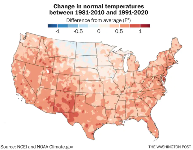
Source: Washington Post
Weather Data
Two types of weather data used by energy efficiency programs and evaluators are heating and cooling degree days (HDD and CDD) and typical meteorological year (TMY) data.
- Cooling degree days measure how warm a location is by comparing the average outdoor temperature to a standard temperature (typically 65°F in the US). Higher outside temperatures result in a higher number of cooling degree days. Heating degree days work the same way, except measuring the temperature below the standard temperature. The energy industry often relies on degree days to estimate the heating or cooling requirements of HVAC equipment. Degree days can be used to normalize energy use for changes in weather, either comparing one year to another or one location to another.
- Typical meteorological year data contains one year of hourly data that best represents “typical” conditions over a multi-year period for a given weather station. For example, if a site has 30 years of data available, NREL analyzed all 30 instances of a given month and then selected the most typical month to include in the data set.[5] The most recent TMY data set (TMY3) is derived data from 1991-2005.[6] For example, a TMY developed from the years X to Y might use data from 2000 for January 2005 for February, etc. TMY allows us to create weather-normalized performance or production estimates to make comparisons across time, locations, and system types.
Programs often base their savings calculations on CDD or HDD values prescribed in their technical reference manuals (TRMs) and/or use TMY3 data. (Sometimes, they even use TMY2, which is based on weather records from 1961-1990.) As described above, using outdated weather data that does not account for recent increases in average temperatures, and can result in inaccurate estimates of energy usage and savings. Below, we use equivalent full load hours (EFLH) to demonstrate this.
Primer on EFLH
Most TRMs calculate savings for residential air conditioning or heat pump systems with an algorithm like this[7]:
kWh Saved = (Size kBtu/hr) * (1/SEERbaseline – 1/SEERinstalled) * EFLHcooling
Where:
Size kBtu/hr – cooling capacity of the unit
SEERbaseline = seasonal energy efficiency ratio of the baseline unit
SEERinstalled = seasonal energy efficiency ratio of the installed high-efficiency unit
EFLHcooling = equivalent full-load hours for cooling
Equivalent full-load hours[8] (EFLH) represent the number of hours per year an AC would have to operate to equal the amount of cooling delivered by the system at a constant thermostat setting over a cooling season. EFLH estimates are typically developed either through building simulations[9] or through equipment metering.[10] EFLH is calculated by dividing the total seasonal energy consumption (kWh) by the nameplate rated peak demand (kW).
EFLH can also be estimated using the following equation:
(CDD * 24 (degree hours))/(design temp °F - 65°F)
Results from metering studies find that the actual EFLHcooling is often lower than values created through building simulations or the above equation. This is likely due to variable weather patterns, manual changes to the thermostat, vacancy, and (over) sizing practices. In colder areas, differences may also result from heat pumps being oversized to meet heating loads.
To illustrate how changing temperature trends may affect EFLH and therefore energy consumption and savings, I reviewed annual CDD values for a selection of states and the United States overall as a proxy for EFLH. The chart below shows the 5-year moving average of annual CDD values to smooth out the natural oscillation of temperatures in each year. Note that these values are population-weighted for each state and that specific location in each state may be quite different than the state average shown.
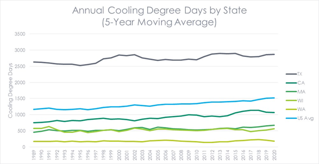
Source: https://www.cpc.ncep.noaa.gov/products/analysis_monitoring/cdus/degree_days/
Looking at this chart, three things stand out to me:
- The cooling degree day values in each of the states shown, as well as for the US overall, increased over the past 30 years. CDDs appear to have increased by about 0.5% to 1% per year since 1989 and about 1% to 2% per year since 2010.
- The increases are not the same for each state. CDD appears to have increased (relatively) the most for Massachusetts and California and least for Wisconsin, Washington, and Texas, although the absolute increase is highest for Texas.
- As expected, different locations have much different cooling needs. Texas has about 15 times the CDD as Washington. This means that the installed cooling equipment and grid requirements will be much different as will the impact of a heatwave on each state.
Impact on Cooling Savings
Let’s focus on an example of Massachusetts. Using a 5-year moving average CDD value of 601 for the year 2017 and a design temperature of 95°F, the estimated EFLHcooling is 481 hours using the CDD equation described above. In 2017, Navigant conducted a residential baseline load shape study and found an EFLHcooling of 419 hours for central AC/heat pump systems and 417 hours for ductless AC/heat pumps. Like other metering studies, the measured EFLH was somewhat lower than the estimated value (13% lower in this case).
If we assume that the annual CDD is increasing in Massachusetts at a rate of about 1% per year, this means that the metered EFLH of 419 hours is now about 436 in 2021 and the savings per system calculated per the MA TRM has increased from 222 kWh to 231 kWh.[11] This may seem trivial, but over the course of the 18-year life of the system, it means the program underestimated lifetime savings by 349 kWh (4,345 kWh vs. 3,996 kWh) or 9% per system. Multiplied over thousands of units over multiple years and it starts adding up.
Of course, this is a very simple example. The actual EFLH of the equipment will not be perfectly aligned with cooling degree days. It will depend on many factors, such as the home's insulation level, humidity, the sizing of the system[12], the frequency of major heatwaves, the building’s internal heat gains, and more. Lastly, we have only looked at cooling – as temperatures increase, the industry may be underestimating cooling and overestimating heating savings.[13]
What does this all mean? Given the rapidly warming climate, we cannot rely on outdated weather data when estimating savings, especially forward-looking lifetime savings. In the past, it may have been possible to use weather assumptions for 10-20 years before they were considered outdated, but that is no longer the case. Weather data and EFLH values need to be revisited and researched regularly. This is especially true for heat pumps, which have both cooling and heating savings and could be affected in both the cooling and heating seasons.
[1] According to the latest NEEA residential baseline study, 35% of single-family homes and 72% of multifamily buildings in the Pacific Northwest do not have cooling equipment.
[2] In these charts, blue represents a lower mean annual temperature than the average for the period and red represents a higher temperature. The darker the color, the farther from average.
[3] 2020 was two for one at the global crisis store!
[4] “The climate is what you expect; the weather is what you get.” – Probably not Mark Twain.
[5] Based on temperature, dew point, wind speed, and solar radiation.
[6] When available for certain locations, data from 1976-2005 were used.
[7] This version is from the Uniform Methods Project.
[8] Much of the information presented in this section has been distilled from an excellent ACEEE paper by David Korn and John Walczyk.
[9] Many jurisdictions use EFLH derived from California’s building simulations and scale it based on CDD.
[10] Notably, the Uniform Methods Project recommends extrapolating metering to the entire year using TMY data, which is problematic if the TMY data is not representative of actual weather.
[11] Using the TRM values of a 2.7 ton 16.5 SEER system compared to a baseline of 13 SEER.
[12] In colder climates like Massachusetts, heat pumps are often oversized to meet the heating load. But if the cooling load increases over the life of the system, maybe they are no longer oversized? Also, TMY or CDD
[13] Or maybe not. Slightly warmer winters may result in more savings for heat pumps which may operate more efficiently.